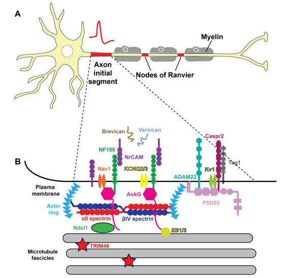
3.7.3 Role of AIS

As we also discussed [26], more interactions are involved in the living matter, and the interactions need a spatiotemporal description. We use the notion of time dependence in the Einsteinian sense: the basic entities such as location and time are connected through their interaction speed and they are not independent parameters in the Newtonian sense. So, we expected that neurons, as dynamical thermoelectricity-based systems, are described by thermoelectric time-dependent equations. However, it is not so.

One of the fundamental reasons is that the way of providing time derivatives of the thermoelectricity process was not known (see our section 2.4.5). The other is that, conceptually, the neuron is considered to be a purely electric system that connects to thermodynamics only through the time-independent Nernst-Planck equation. The third is that even the description of the purely electric operation is wrong: biology separated the primary abstraction of electric ’charge’ from its secondary manifestations of abstractions ’potential’ and ’current’; furthermore, it assumes that a mysteric power changes biological ’conductance’ against all physics laws (applying laws of electricity to their ’non-ohmic’ systems). The fourth is modeling problems we discuss below. Theory of biology, among others, stayed at its century-old ideas about equipotential neuron surface, time-unaware information processing [16], although the experimental physiology delivers a vast amount of evidence for the opposite.

By assuming that biological operation can be described by well-known electric terms, Hodgkin and Huxley [9] advanced neuroscience enormously. However, their seven-decades-old hypotheses must be updated from several points of view. Among others, they provided a static empirical description (their differential equations rely on derivatives of an empirical function fitted to empirical measurement data, and even in a wrong way). They excluded interpreting the physical background of their empirical description using an empirical conductance function; in this way, really, there is “little hope of calculating .. from first principles”. Their suggestion about equivalent circuits introduced the idea that the membrane’s potential remains unchanged during operation despite the ion traffic, the ions in the current do not affect concentration, and the components of the circuit operate with the speed of the EM waves. By introducing the delayed current and that some mystic power controls the operation of neurons by changing their conductance, they gave way to introducing the fallacy that science and life sciences are almost exclusive fields. Furthermore, their (unintended) model provokes questions (for a review see [68]) whether it is model at al and what controversies it delivers.

They meticulously wrote that “the success of the equations is no evidence in favour of the mechanism … that we tentatively had in mind when formulating them”. Although “certain features of our equations were capable of a physical interpretation”, “the interpretation given is unlikely to provide a correct picture of the membrane”. Despite their doubts, biophysics produced fictitious mechanisms to underpin their equations, describing an admittedly wrong physical picture instead of setting up a correct physical operation and describing the processes by deriving physically plausible approximations and using correct mathematical expressions. Although they warned that “the agreement [between our theory and experiments] must not be taken as evidence that our equations are anything more than an empirical description”, their followers forgot their doubts and question marks and took their unproven hypotheses as facts. ”These equations and the methods that arose from this combination of modeling and experiments have since formed the basis for every subsequent model for active cells. The model and a host of simplified equations derived from them have inspired the development of new and beautiful mathematics.”[45]. However, there was no model, and the beautiful mathematics describes a fictitious neuron.

One of the most influencing bad ideas was expressed by their Eq.(1). In their time, at that limited microscope resolution, they did not see any structure within the neuron’s membrane, so logically, they assumed that the measured capacitance and resistance were distributed. Correspondingly, they introduced an electric equivalent circuit assuming that the neuronal $RC$ circuit comprised parallelly connected discrete $R$ and $C$ elements. They described the neuronal operation as based on an integrator-type equivalent electric circuit with the corresponding equations.

They assumed that a fixed voltage drives a constant current through the circuit, and the discrete $R$ and $C$ elements share that current. Correspondingly, a leaking current must exist, and the resting brain must dissipate power (as later estimated, around $20W$). However, the operation of the neuronal circuit resulted in well-measurable hyperpolarization (the output voltage changes its sign), which the equivalent parallel electric circuit cannot produce, so they assumed that in addition to a $N{a}^{+}$ current, a delayed $K^{+}$ current to flow through the neuron membrane in the opposite direction, against the flow of $N{a}^{+}$ ions. In their milestone work, their goal was to derive equations for practical application, so they introduced equations describing the measured electric observations. Unfortunately, they attempted to determine which processes were going on inside the biological neuron.

In the past years, instrumental advances have enabled us to discover the “white spots” of their time. Around 2018, the AIS was discovered and understood [54, 50]. From an electric point of view, the AIS is an array of ion channels with well-measurable resistance; it can be abstracted as a discrete resistance. As the anatomical evidence shows, see Fig. 3.8, the currents flow into the membrane and flows out through the AIS. The currents are not shared, and even, the output current cannot directly be concluded from the sum of the input currents: the charge is temporarily stored by the membrane (as a distributed condenser). The correct equivalent circuit is one in which the condenser and resistor are switched in serial (although the resemblance has limitations), that is a differentiator-type electric circuit. This circuit is sensitive to voltage gradient, so the rising and falling edges of an input signal (such as a PSP) can natively produce an opposite voltage on its output, making the need (and the existence) of the assumed delayed $K^{+}$ current at least questionable. Also, a recent measurement [78] concluded that the neuronal computation (contrasted with the resting state) needs only $0.1W$ and neuronal communication needs only $3.5W$; that is, the leaking current, at least due to the parallel $RC$ circuit, does not exist (see our Figure 3.9: a current flows only if membrane’s potential is above the resting potential).

We know from the recent discoveries and understanding of the correct model that currents flow into the condenser (the membrane) and are taken out through the resistor (the AIS). Our theoretical discussion solidly underpins that the physical picture behind the commonly accepted neuronal electric model must be fixed. As we discussed, unlike in the classic model, the driving voltage and the membrane current have a time course. No current is shared by the resistor and condenser, there is no input resistance, resting current of the parallel oscillator, delayed $K^{+}$ current, and changing conductance.

The correct equivalent circuit is a differentiator-type oscillator, where the output voltage is given by the equation

The sum of all input voltage gradients generates the output voltage, which drives a current through the AIS. The fundamental difference between the two circuit types, that in the correct circuit there is no shared current and there is no direct correction between the input and the output currents. Instead, in the dynamic picture, the changes in the input charge (the temporal course of the current) generates a resulting voltage gradient and their sum drives the $RC$ circuit, which (under its laws) generates the output voltage which drives a current (pulse) though the AIS Here comes to light the biggest mistake in deriving HH’s equations: the temporal course of the charge is identical with the current only if the current is constant such as in the case of clamping.

As we derived, the (the measured AP) output voltage can be described by the equation describing the serial $RC$ circuit. Our equations enable us to calculate the ion current’s time course from the potential’s time derivative. We need to sum the time derivatives of the voltages that drive the neuronal oscillator through its membrane (of course, considering that the current needs time to travel from its entry point to the membrane’s body) and solve the differential equation by integrating it in time. The resulting output voltage time derivative can be measured in front of and after the AIS. Interestingly, the time derivative was measured as early as 1939 [43], but its role has not been understood, mainly due to the wrong electric model. The causality is reversed. The voltage gradient is the primary entity produced by the cellular circuit, and that leads to the production of an AP by the neuronal oscillator.

Figure 3.9 shows how the described physical processes control neuron’s operation. In the middle inset, when the membrane’s surface potential increases above its threshold potential due to three step-like excitations opens the ion channels, $N{a}^{+}$ ions rush in instantly and create an exponentially decreasing, step-like voltage derivative that charges up the membrane. The step-like imitated synaptic inputs are resemblant to the real ones: the incoming PSP s produce smaller, rush-in-resemblant, voltage gradient contributions. The charge creates a thin surface layer current that can flow out through the AIS. This outward current is negative, and proportional to the membrane potential above its resting potential. At the beginning, the rushed-in current (and correspondingly, its potential gradient contribution) is much higher than the current flowing out through the AIS, so for a while the membrane’s potential (and so: the AIS current) grows. When they get equal, the AP reaches its top potential value. Later the rush-in current gets exhousted and its potential-generating power drops below that of the AIS current, the resulting potential gradient changes its sign and the membrane potential starts to decrease.

In the previous period, the rush-in charge was stored on the membrane. Now, when the potential gradient reverses, the driving force starts to decrease the charge in the layer on the membrane, which per definitionem means a reversed current; without foreign ionic stream and current through the AIS. This is the basic difference between the static picture that Hodgkin and Huxley hypothesized and the dynamic one that really describes its behavior. The correct equivalent electric circuit of a neuron is a serial, instead of a parallel, oscillator, and its output voltage is defined dynamically by its voltage gradients (see Eq.(3.2)) instead of static currents (as physiology erroneously assumes). In the static picture the oscillator is only an epizodist, while in the time-aware (dynamic) picture it is a star.

Notice also that only the resulting $\frac{dV}{dt}$ (APTD) disappears with the passing time. Its two terms are connected through the membrane potential. As long as the membrane’s potential is above the resting value, a current of variable size and sign will flow, and the output and input currents are not necessarily equal: the capacitive current changes the rules of the game.

The top inset shows how the membrane potential controls the synaptic inputs. Given the ions from the neuronal arbor [84, 85] can pass to the membrane using ’downhill’ method, they cannot do so if the membrane’s potential is above the threshold. The upper diagram line shows how this gating changes in the function of time.

Fig. 3.13 shows how the resulting APTD controls the output APs shape: the derivative changes its polarity by $\approx 500mV/ms$ in $\approx 0.5ms$, which means across a $50\mu m$ AIS a $20,000V/m$ gradient change on the AIS. This voltage gradient is sufficient to accelerate the ions in the ion channels and decelerate them again; this is how to reverse the current direction. We see the effect of ’ram current’ as AP. Notice the broadening effect of the gradient measuring technology. A voltage difference is measured at a distance difference, and – due to the signal’s speed – the time difference is comparable in size to the period of polarity change of the signal.