3.8.5 Electricity

The biological ’equivalent circuit’ models assume that the circuits comprise point-like ideal discrete elements such as condensers and resistors, and some hidden power changes their parameters according to some mathematical formulas, furthermore ideal batteries with voltage that may again be changed by that power. All they are connected by conducting (metallic) ideal wires and their interaction speed is infinitely high (the Newtonian ’instant interaction’). Using that abstract model enables them to use the well-known classic equations, named after Ohm, Kirchoff, Coulomb, Maxwell and others. However, those abstractions have severe limitations. Biology applies Ohm’s Law to its objects while claims that its objects are non-ohmic; understands that neural currents comprise ions while claims that the ions do not feel the Coulomb repulsion; measures ions’ propagation speed but in its equations it claims that their effects are instant; hypotesizes non-existing physical mechanisms to make their nature. In in general, biophysics abstracts from the world of the physics-inspired mathematical formulas a fictitious nature where biology lives and hypothesises complementary mechanisms to achieve some resemblance with the true biological word. The examples include that ions in the ions channels do not repulse each other; that charge, potential and current are independent of each other; that ion currents do not repulse each other neither when they travel from the presynaptic terminal to the AIS; that some hidden power opens the ion channels to let ions in into the intracellular space, that ions with the same charge move in opposite directions when ions rush-in into the intracellular segment of the neuron; that the ions pass ion channels without being accelerated by the potential difference accross the membrane; the telegraph equations are applied to the case of axons although neither external potential nor current loss exists; and so on.

Even that unfortunate idea of equivalent circuits leads to analyzing ”electrotonic (electronic circuit equivalent) modeling of realistic neurons and the interaction of dendritic morphology and voltage-dependent membrane properties on the processing of neuronal synaptic input” [47]; that is, to study a simulated neuron built from discrete electronic components. However, the idea needs to put together many compone ”raises the possibility that the neuron is itself a network”. On the one side, such an idea misguides the neurophysical research (since actually a fake neural system is scrutinized, the validity of the approach is questionalized [48]), and on the other, since electroengineers understand the neuronal operation from the wrong model, it also misguides building neuromorphic architectures.

The equivalent circuits are a source of misinterpretations. As [2] formulates, ”In other words, the ionic concentration gradients act like DC batteries for cross-membrane currents.” We call the attention again, that ions represent the current, that is that current changes changes the concentration, that changes the voltage of the DC battery, unlike in the case of the equivalent circuits. This difference is significant in understand how the basic neuronal circuit works. Introducing equivalent circuits prevents explaining the fundamental electric phenomena.

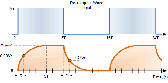
If we apply a continuous square wave voltage waveform to an integrator-type electric RC circuit, we receive an output wave form shown in Fig. 3.18. After switching a voltage to the circuit, a charge-up process starts, then the output voltage saturates. After switching the voltage off, the condenser discharges. The time constant $\tau$ for the charge and discharge processes are identical. If the time period of the input square wave waveform is made longer (in the figure with a half-period “$8\ast \tau$”), the capacitor would then stay fully charged longer and also stay fully discharged longer.

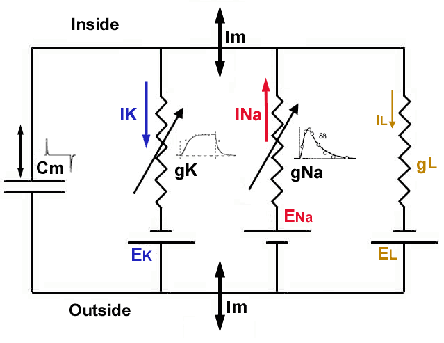
HH measured [9] the time course of the neuronal membrane (i.e., a neuronal $RC$ circuit) when switched clamping axonal voltage on and off. Their measurement result is shown in Fig. 3.19. They experienced a formal similarity with switching a voltage of an integrator-type $RC$ circuit on and off, compare to Fig. 3.18, so they concluded that the response of the neuronal circuit is identical to that of the integrator-type electric $RC$ circuit (see our discussion in sections 2.5.6 and 2.5.6). They (mistakenly) concluded that the electric equivalent circuit of a neuron is a parallelly switched electric $RC$ oscillator. One more evidence that ”the success of the equations is no evidence in favour of the mechanism that we tentatively had in mind when formulating them”.

Figure 3.19 shows two switch-on diagram lines, with two different $\tau$ time constants. The blue line (”electric”) is drawn with the measured time constant of the swith-off discharge. Acconding to the theory of electricity, the time constants of the falling and rising edge must be the same in the case of an electric integrator. The green diagram line (the one fitted to the measured data) correspond to a different $\tau$ time constant. The effect was observed by  [9], but they did not explain and also did not interpret it. Although their fitted polynomial nearly hides the effect, a little ”hump” at around $3ms$ can be observed. The reason is that the charge-up current is not constant, it also has a time course; despite that they stabilized the voltage.

The different time constants should have been a warning sign for HH that the measured effect differs from the one they had in mind. They wanted to believe and demonstrate that they have measured the output signal of a serial $RC$ circuit. With the evaluation of their measurement, they suggested some wrong hypotheses

• •

  They misidentified the current as the change of conductance. No conductance change happens, only a condenser changes and discharges. They worked with a condenser, not with a resistor.

• •

  They meticulously observed and measured that the time contants $\tau$ of the exponential charge-up and discharge processes are different; but did not care that they should be indentical and also did not care of the ”hump”.

• •

  They measured the resulting charge-up composite process. As we explain in section 2.5.2, before switching the clamping voltage, there is no charge carrier inside the axonal tube; first, the ions must diffuse into the axon.

• •

  They fitted the rising time course with a polynomial, hiding that it comprises a saturating voltage of the condenser, that the current through the axon also saturated with a different time constant, and at the begining the line had a zero current contribution.

On the one side, they underpinned that our equations 2.38 and 2.37 describe correctly the axonal chargeup current and discharge currents, respectively. On the other, as they noticed that the time constants of the two processes are significantly different (see the green and the dashed blue diagram lines), underpinned that the axonal charge production mechanism significantly changes the axonal source current. The green line has significantly slower rise since the axonal current only gradually increases after switching the clamping on. Without that current change, the charge-up current would follow the blue line. Unfortunately, there are three physical processes, with similar time constants. One, that they wanted to demonstrate is the steady state: the current leads to a saturated current. Two, that the clamping ”creates” charge carriers in the axon, so the charging current changes. Three, the initial switch-on creates a voltage gradient on the membrane, so an action potential is also started.

Their equations more or less precisely describe the features of the wrong oscillator type and those of the non-existing $K^{+}$ current introduced for compensating for the wrong oscillator selection.

Selecting the wrong oscillator type (actually, assuming distributed parallel oscillator circuit) and the wrong electrotonic model leads to somewhat surprising consequences, such as using the telegrapher equations in a wrong way for describing neuronal transfer. By using the cable equation, as Hodgkin and Huxley attempted [9], led to numerical difficulties, and they faced the principal problem: their equations assumed infinitely fast electric interaction, and they attempted to combine them with the (unknown) finite macroscopic speed of current in neuronal telegraph cables. The validity of using cable equations for biological objects is at least doubtful: deriving a telegrapher equation assumes applying an external potential to the cable filled with charge carriers, and in the case of biological membranes neither external potential nor permanently present charge carriers exist. Furthermore, the cable equation assumes continuous current outflow (a distributed resistance), which is not true for the neuronal membrane (current flows only toward the AIS).