2.6 Electrolyte’s electricity 2.6.3 Thermodynamic field 2.6.5 Two segments

2.6.4 One segment

We prepare a tiny electrolyte volume filled with a solution containing ions (such as $Na^{+}$ , $K^{+}$ and $Ca^{+}$ ; furthermore, of course $Cl^{-}$ or similar). The overwhelming majority of those ions is chemically bound, but a minority might exist separately from each other; especially under external macroscopic changes applied to the volume. For the discussion below, we assume that the segment has a two-dimensional surface boundary (see Fig. 2.9) and we discuss the gradients along a line, perpendicular to that plane surface. We compose the segments from such layers (sheets), $(x,y)$ parallel plates, and describe the gradients in direction of $z$ . Having the membrane’s shape in mind, we introduce the idea of ’thin physical layer’, that is parallel with the membrane and has a finite width. We compose the segments from such layers having different potentials.

In the calculations below, we need the notion of ’surface charge density’ (interpreted for an ’infinitely thin layer’ in physics; given in $C*m^{-2}$ ). We know that $1\ mM$ concentration means that $6.023*10^{20}$ atoms are present in $1\ m^{3}.$ We can derive (assuming singly-charged ions) the volume charge density (the concentration $c$ is given in $m M$ )

	$\displaystyle\sigma_{V}(c)$	$\displaystyle=$	$\displaystyle cN_{A}e_{el}=c6.02310^{20}1.60210^{-19}$		(2.56)
		$\displaystyle=$	$\displaystyle 96.4c\quad\biggl{[}\frac{C}{mMm^{3}}\biggr{]}$		(2.57)

where $N_{A}$ is the number of ions in a $m i l l i m o l$ and $e_{el}$ is the elementary charge. By assuming an arbitrary ’physical ion layer thickness’ $\Delta z$ we can calculate the surface charge density $\sigma_{A}(\Delta z)$ we need for our calculations below as

\sigma_{A}(c,\Delta z)=96.4*c*\Delta z\quad\biggl{[}\frac{C}{mM*m^{2}}\biggr{]}

(2.58)

Below, we interpret classical physics’s notions from the theory of ’continuous’ electricity, interpreted for ’infinite’ cases, for the finite world of biological objects (’living matter’) and the atomic world of ions. We know the permittivity of free space

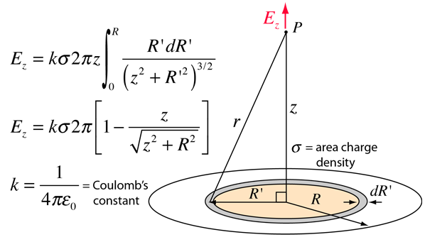
\epsilon_{o}=8.854*10^{-12}\quad\biggl{[}\frac{C}{V*m}\biggr{]}

From the theory of electricity we know that a charged layer generates a field

E_{z}(c,\Delta z)=\frac{\sigma_{A}(c,\Delta z)}{2*\epsilon_{o}}=5.45*10^{3}*c*% \Delta z\quad\biggl{[}\frac{V}{m}\frac{1}{nm*mM}\biggr{]}

(2.59)

We assume that when ions are present in an electrolyte having concentration $c$ in a ’conducting layer’ of thickness $\Delta z$ on an isolating surface, they produce such an electrical field. Furthermore, we assume that the electrical field is formed (after integrating the contributions of the rings over the surface) as shown in Fig. 2.10 (for deriving that equation, see section 2.6.5). Notice that here we run into conflict between the ’infinitely thin’ layer of physics and the biologically implemented (finitely) ’thin physical layer’, so we use a thickness parameter $\Delta z$ .

Refer to caption — Figure 2.10: The electrical field of a disc of charge can be found by superposing the point charge fields of infinitesimal charge elements. This can be facilitated by summing the fields of charged rings.